CH 4   2-D Steady State Conduction      Numerical Solution of HE (finite-difference) example 

>

restart;

 

>	with(linalg):

 

Warning, the protected names norm and trace have been redefined and unprotected
 

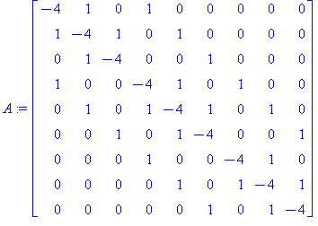
>	A:=matrix([[-4,1,0,1,0,0,0,0,0],[1,-4,1,0,1,0,0,0,0],[0,1,-4,0,0,1,0,0,0],[1,0,0,-4,1,0,1,0,0],[0,1,0,1,-4,1,0,1,0],[0,0,1,0,1,-4,0,0,1],[0,0,0,1,0,0,-4,1,0],[0,0,0,0,1,0,1,-4,1],[0,0,0,0,0,1,0,1,-4]]);

 

>	b:=matrix([[-30.],[-20.],[-70.],[-10.],[0.],[-50.],[-40.],[-30.],[-80.]]);

 

>	x:=linsolve(A,b);

 

>	with(plots):

 

Warning, the name changecoords has been redefined
 

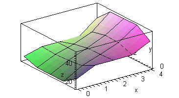
>	TF:=[[[0,0,20],[1,0,30],[2,0,30],[3,0,30],[4,0,40]],[[0,1,10],[1,1,22],[2,1,29],[3,1,36],[4,1,50]],[[0,2,10],[1,2,20],[2,2,28],[3,2,37],[4,2,50]],[[0,3,10],[1,3,19],[2,3,25],[3,3,33],[4,3,50]],[[0,4,15],[1,4,20],[2,4,20],[3,4,20],[4,4,35]]]:

 

>	surfdata(TF,axes=boxed,labels=[x,y,z]);